Model monitoring

H2O MLOps model monitoring involves observing the performance and behavior of deployed models to ensure they continue to operate effectively and to identify issues such as model drift.

This guide explains how to configure model monitoring during deployment, analyze aggregated data, and identify model drift. Follow the steps below to set up and use model monitoring in H2O MLOps.

Model monitoring with the UI

Step 1: Enable model monitoring

To enable model monitoring for your deployment:

1. In the left navigation panel, click Real-time deployments.
2. Click Create deployment.
   
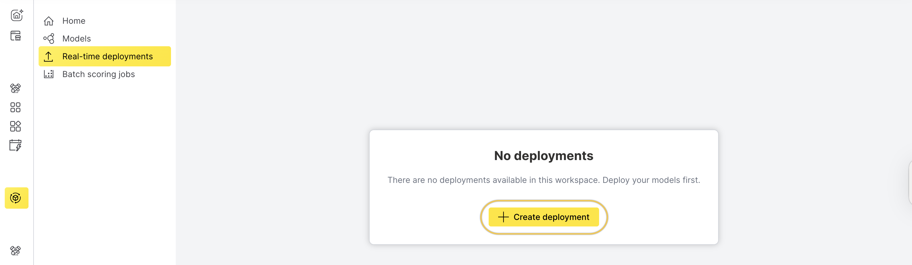
3. On the Create new deployment page, click Advanced settings.
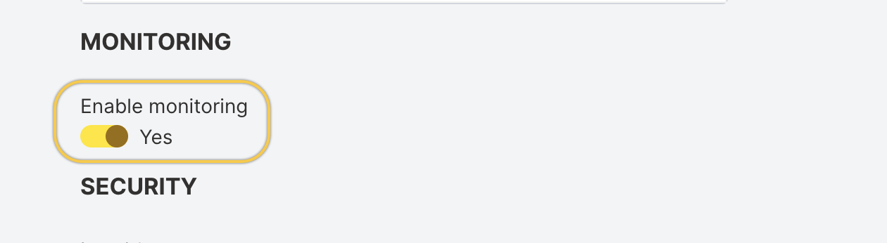
4. Toggle Enable monitoring to Yes.
   

Step 2: Configure and deploy

During model deployment, configure monitoring to collect and analyze data.

1. If Kafka is available in your environment, provide a pre-created Kafka topic where raw data will be sent.
   For more information, see Raw data export to Kafka.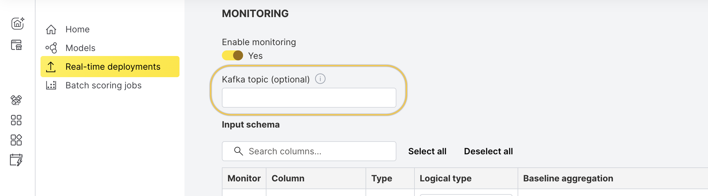
2. Select the columns you want to monitor.
   
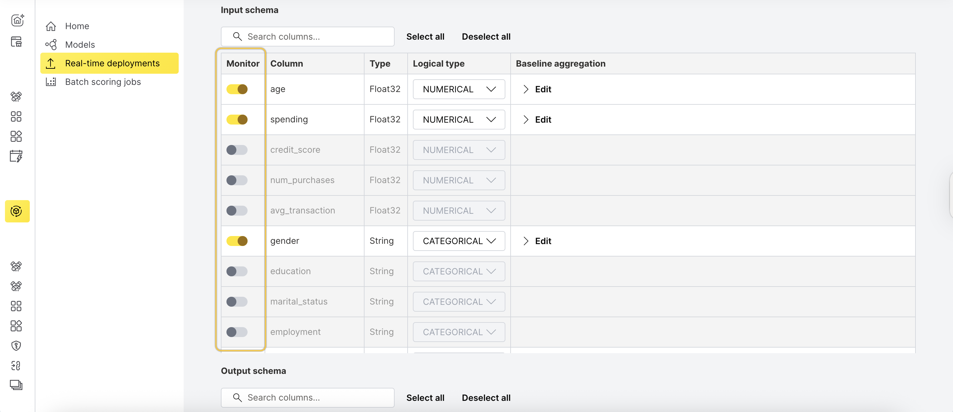
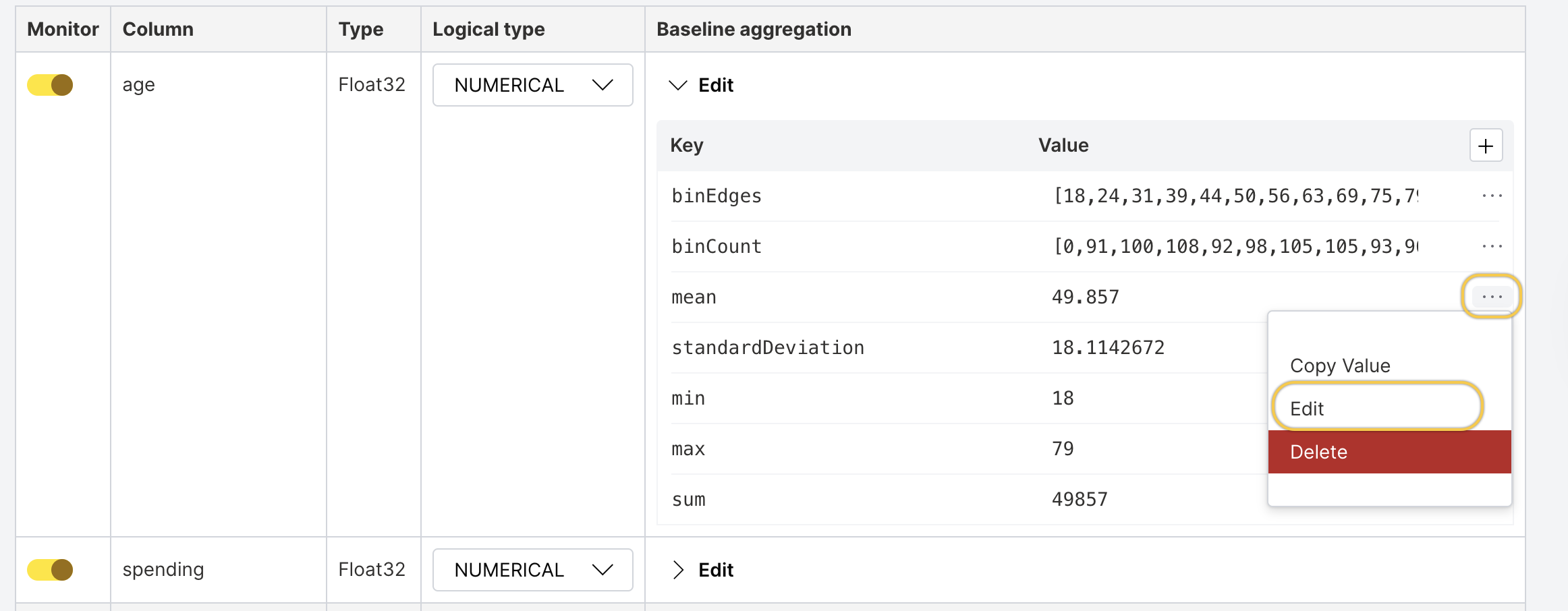
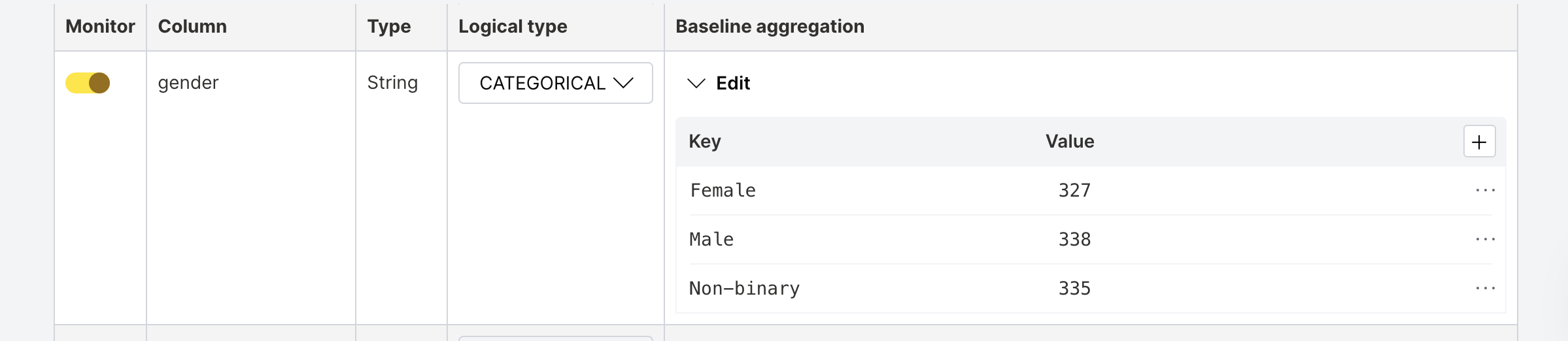
3. Provide baseline data for comparison:
   • Numerical features:
   • Categorical features:
4. Click Deploy.

Step 3: Start scoring

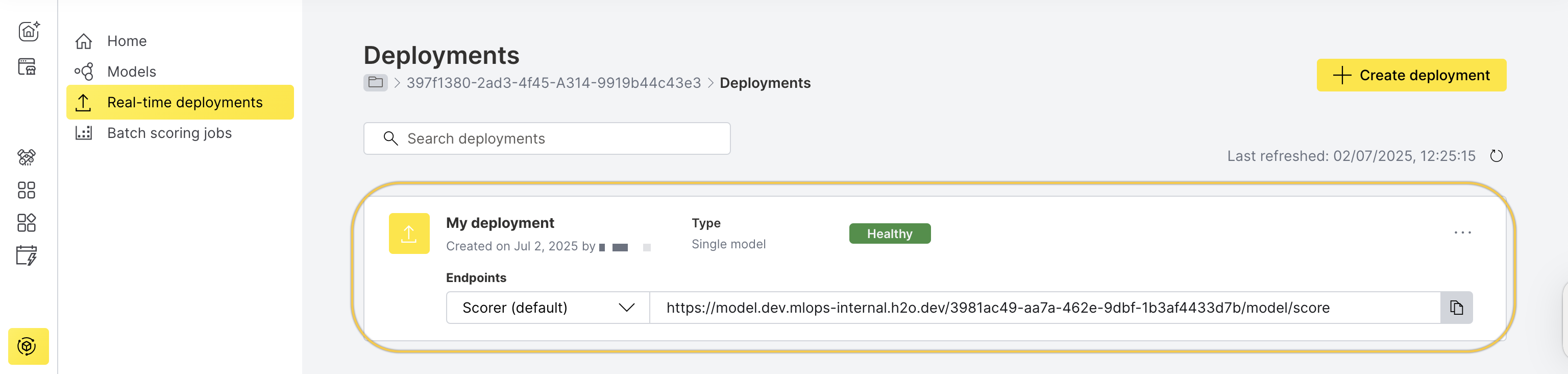
Once the deployment is Healthy, you can begin scoring.

1. In the left navigation panel, click Real-time deployments.
2. Select the deployment you created.
   
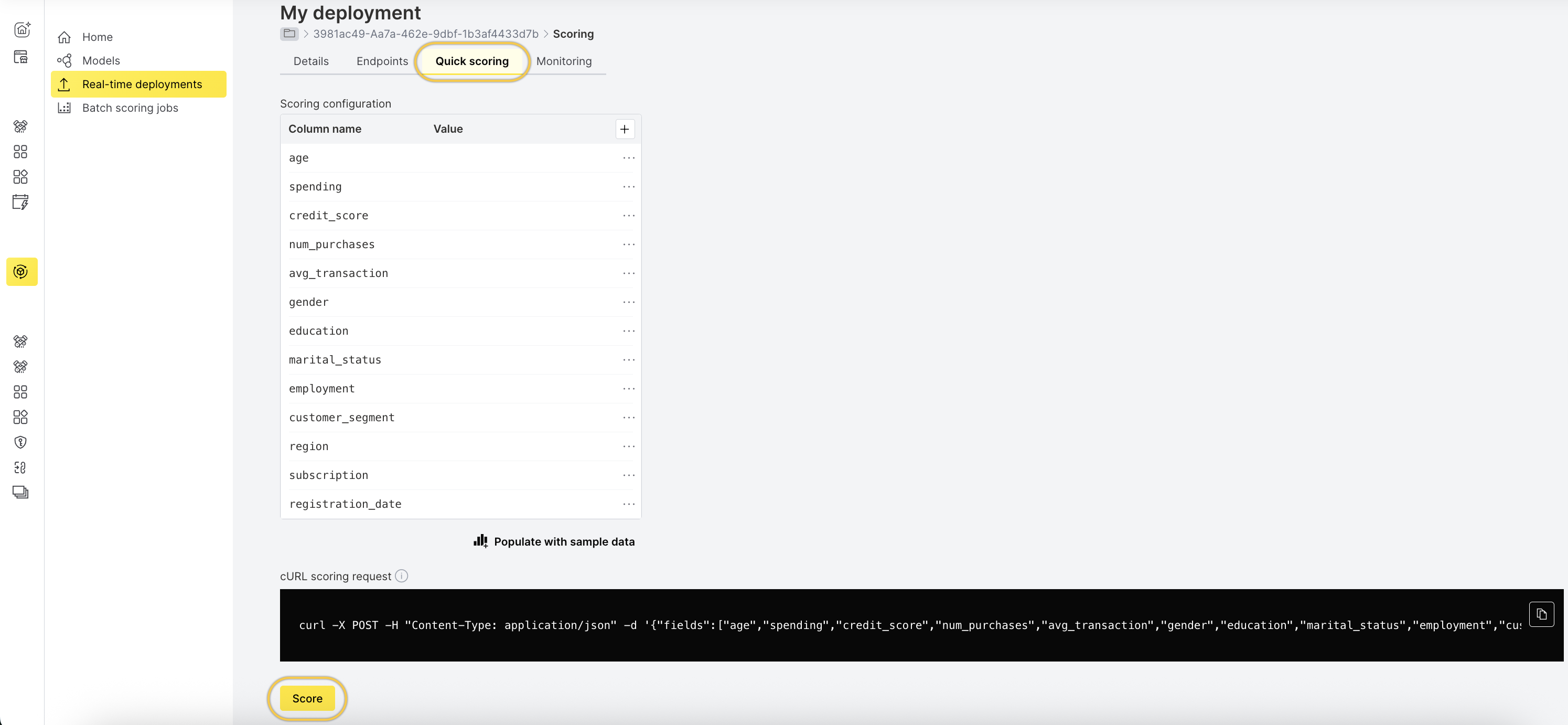
3. Go to the Quick scoring tab.
4. Click Score.

Step 4: View aggregated data

To view the scoring aggregates for each monitored column:

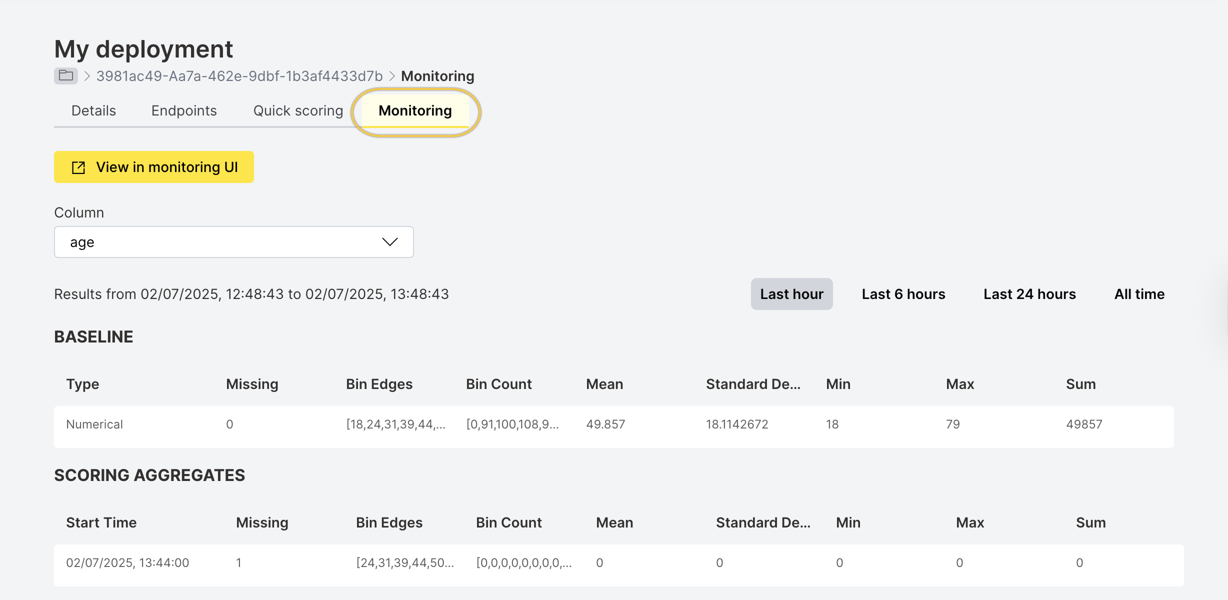
1. After scoring completes, go to the Monitoring tab.
2. Wait 3–5 minutes to see data under Scoring aggregates.

Step 5: Analyze data in the monitoring UI

To view and analyze model drift:

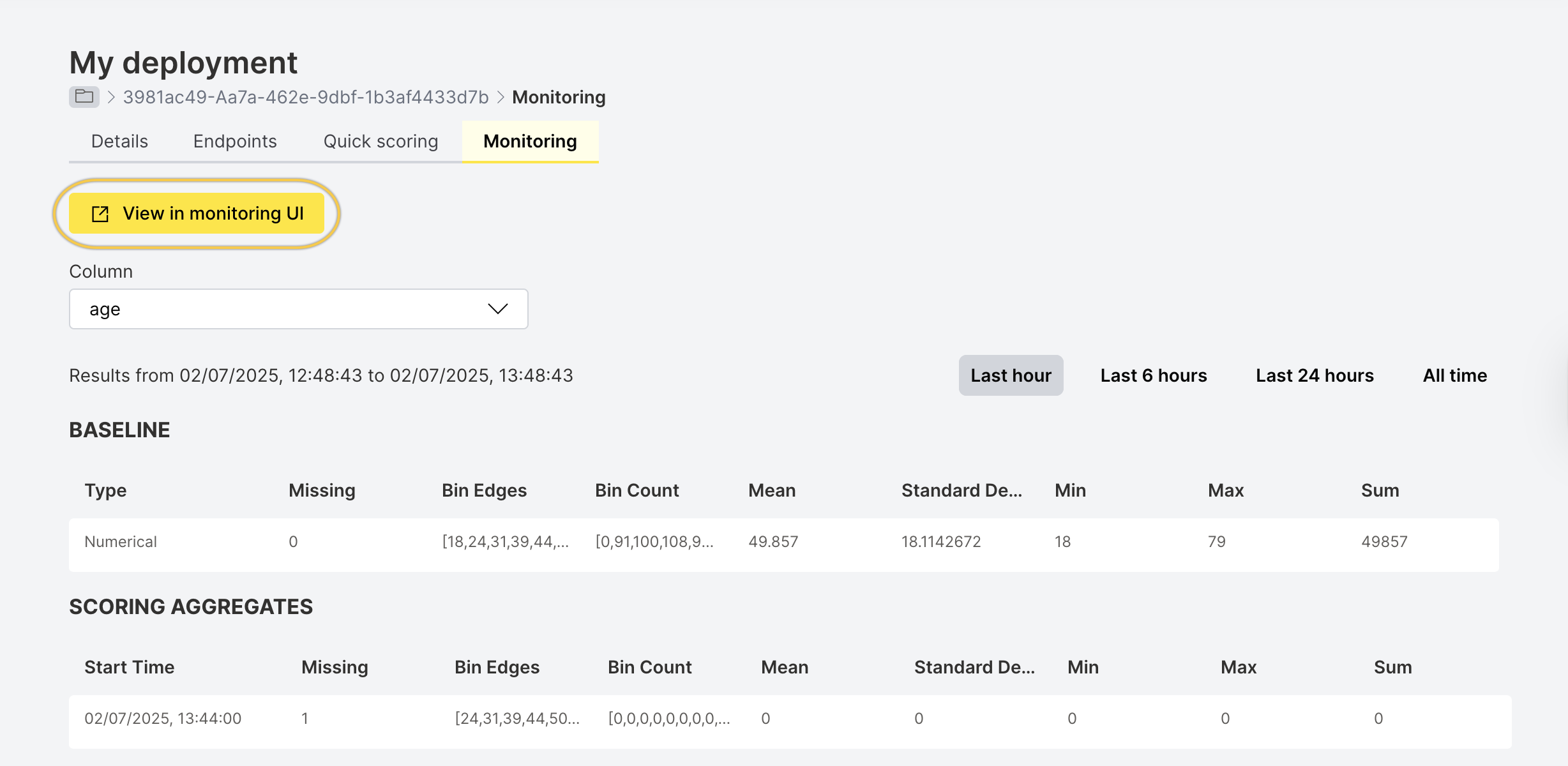
1. Click View in monitoring UI.

2. The Superset UI opens.

3. From the SQL drop-down, select SQL Lab.

4. Schema and table selection:

   • Schema name is the Workspace ID from the H2O AI Cloud Workspaces UI. Copy the Workspace ID and select that schema in Superset. See Workspaces in H2O AI Cloud.
   • Table name is the Deployment ID. From the MLOps Deployments page, copy the deployment ID (it appears in the default scorer URL). In Superset, select the table named aggregates_<deployment_id>.
   • Alternatively, in SQL Lab, use the dropdowns labeled Schema and See table schema to choose the workspace (schema) and aggregates_<deployment_id> (table).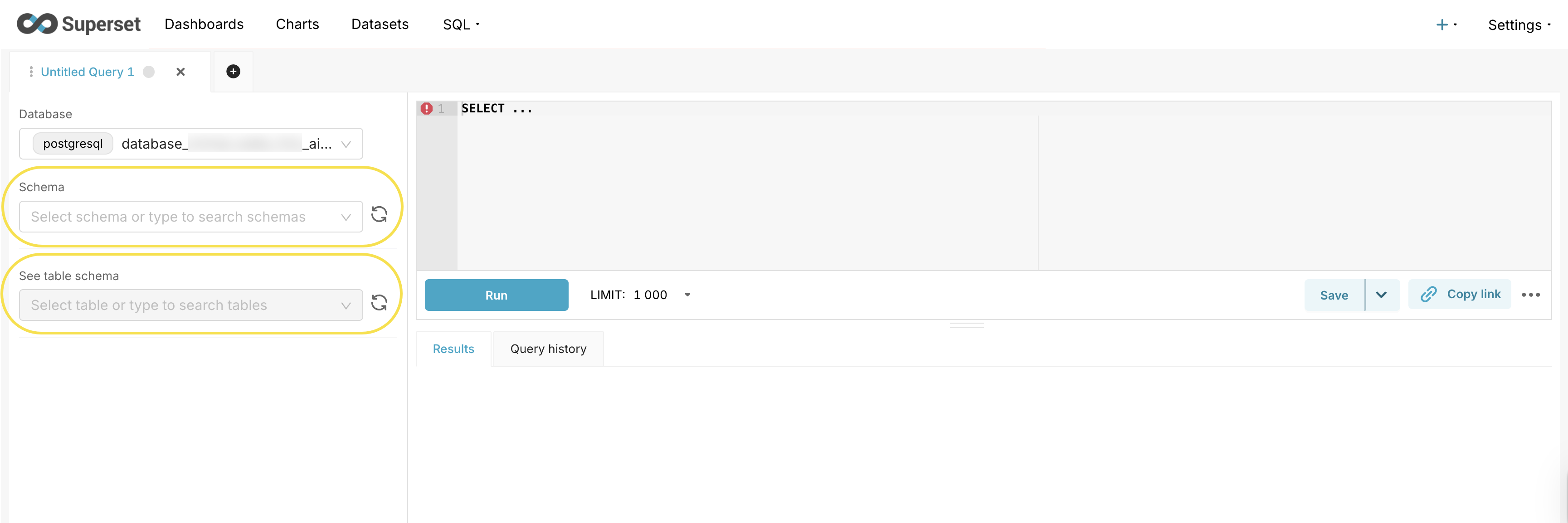

5. Enter the drift query:
   Example:

   WITH time_series AS (
   -- Get all unique timestamps for the series
   SELECT DISTINCT "timestamp"
   FROM <TABLE_NAME>
   WHERE NOT is_baseline
   AND column_name = <FEATURE_NAME>
   ORDER BY "timestamp"),
   baseline AS (
   -- Get the baseline (expected) data
   SELECT unnest(bin_counts) as count
   FROM <TABLE_NAME>
   WHERE is_baseline
   AND column_name = <FEATURE_NAME>),
   baseline_sum AS (
   -- Calculate sum of baseline counts
   SELECT sum(count) as total
   FROM baseline),
   baseline_props AS (
   -- Calculate baseline proportions
   SELECT count / total        as prop,
   row_number() OVER () as rn
   FROM baseline,
   baseline_sum),
   actual_data AS (
   -- Get actual data for each timestamp
   SELECT "timestamp",
   unnest(bin_counts)                            as count,
   row_number() OVER (PARTITION BY "timestamp") as rn
   FROM <TABLE_NAME>
   WHERE NOT is_baseline
   AND column_name = <FEATURE_NAME>),
   actual_sums AS (
   -- Calculate sums for each timestamp
   SELECT "timestamp",
   sum(count) as total
   FROM actual_data
   GROUP BY "timestamp"),
   actual_props AS (
   -- Calculate proportions for actual data
   SELECT a."timestamp",
   a.count / s.total as prop,
   a.rn
   FROM actual_data a
   JOIN actual_sums s ON a."timestamp" = s."timestamp"
   WHERE s.total >= 0 -- Implementing the Python None return for sum < 200
   ),
   drift_calc AS (
   -- Calculate absolute differences and sum them
   SELECT a."timestamp",
   sum(abs(a.prop - b.prop)) / 2 as drift_score
   FROM actual_props a
   JOIN baseline_props b ON a.rn = b.rn
   GROUP BY a."timestamp")
   -- Final result with timestamps and drift scores
   SELECT "timestamp",
   drift_score
   FROM drift_calc
   ORDER BY "timestamp";

   Additional Examples:

   General numerical columns drift query with time window aggregation:

   -- Replace '<TABLE_NAME>' with your table of interest
   -- Drift calculation for all numerical columns:
   -- Corrected to avoid false drift for identical distributions
   -- Numerical drift with time window aggregation for small samples
   -- This query aggregates bin_counts across time windows before calculating drift
   -- **CHANGE THIS LINE** to adjust aggregation window: 'hour', 'day', 'week', 'month'
   -- 'minute' - Aggregates all records within the same minute
   -- 'hour' - Aggregates all records within the same hour, please use it if small number of data. It's default.
   -- 'day' - Aggregates all records within the same day
   -- 'week' - Aggregates all records within the same week
   -- 'month' - Aggregates all records within the same month
   
   WITH base_raw AS (
       SELECT
           column_name,
           "timestamp",
           DATE_TRUNC('minute', "timestamp") AS time_bucket,
           is_baseline,
           bin_counts,
           bin_edges
       FROM <TABLE_NAME>
       WHERE logical_type = 1
         AND bin_counts IS NOT NULL
         AND bin_edges IS NOT NULL
   ),
   
   -- Expand baseline bins with correct ordering by bin_edges
        baseline_expanded AS (
            SELECT
                column_name,
                row_number() OVER (PARTITION BY column_name ORDER BY bin_edges_array) AS bin_position,
                bc_value::numeric AS count  -- CAST the value, not the record
            FROM base_raw,
                 LATERAL unnest(bin_counts) WITH ORDINALITY AS bc(bc_value, bin_index)
                     CROSS JOIN LATERAL (SELECT bin_edges[bin_index] AS bin_edges_array) AS e
            WHERE is_baseline = TRUE
        ),
   
   -- Sum baseline counts per column
        baseline_sum AS (
            SELECT column_name, SUM(count) AS total
            FROM baseline_expanded
            GROUP BY column_name
        ),
   
        baseline_norm AS (
            SELECT
                b.column_name,
                b.bin_position,
                b.count::numeric / NULLIF(s.total, 0) AS prop
            FROM baseline_expanded b
                     JOIN baseline_sum s USING (column_name)
        ),
   
   -- Distinct timestamps for actual data
        time_buckets AS (
            SELECT DISTINCT column_name, time_bucket
            FROM base_raw
            WHERE is_baseline = FALSE
        ),
   
   -- Expand actual bins with correct ordering by bin_edges
        actual_expanded AS (
            SELECT
                a.column_name,
                a.time_bucket,
                row_number() OVER (PARTITION BY a.column_name, a.time_bucket ORDER BY bin_edges_array) AS bin_position,
                bc_value::numeric AS count  -- CAST the value, not the record
            FROM base_raw a,
                 LATERAL unnest(a.bin_counts) WITH ORDINALITY AS bc(bc_value, bin_index)
                     CROSS JOIN LATERAL (SELECT bin_edges[bin_index] AS bin_edges_array) AS e
            WHERE a.is_baseline = FALSE
        ),
   
   -- Sum actual counts per column & time bucket
        actual_sum AS (
            SELECT column_name, time_bucket, SUM(count) AS total
            FROM actual_expanded
            GROUP BY column_name, time_bucket
        ),
   
   -- Combine baseline bins with all actual time buckets
        baseline_with_times AS (
            SELECT
                t.column_name,
                t.time_bucket,
                b.bin_position,
                b.prop AS baseline_prop
            FROM time_buckets t
                     CROSS JOIN baseline_norm b
            WHERE t.column_name = b.column_name
        ),
   
   -- Compute actual proportions, default 0 if missing
        actual_norm AS (
            SELECT
                bwt.column_name,
                bwt.time_bucket,
                bwt.bin_position,
                COALESCE(ae.count::numeric / NULLIF(s.total, 0), 0) AS actual_prop,
                s.total AS sample_size,
                bwt.baseline_prop
            FROM baseline_with_times bwt
                     LEFT JOIN actual_expanded ae
                               ON bwt.column_name = ae.column_name
                                   AND bwt.time_bucket = ae.time_bucket
                                   AND bwt.bin_position = ae.bin_position
                     LEFT JOIN actual_sum s
                               ON bwt.column_name = s.column_name
                                   AND bwt.time_bucket = s.time_bucket
        ),
   
   -- Drift calculation (TVD)
        drift_calc AS (
            SELECT
                column_name,
                time_bucket,
                0.5 * SUM(ABS(actual_prop - baseline_prop)) AS drift_score,
                MAX(sample_size) AS sample_size,
                COUNT(*) AS num_bins
            FROM actual_norm
            GROUP BY column_name, time_bucket
        )
   
   SELECT
       column_name,
       time_bucket AS timestamp,
       ROUND(drift_score::numeric, 4) AS drift_score,
       CASE
           WHEN sample_size IS NULL OR sample_size < 3 THEN 'Insufficient Data'
           WHEN drift_score < 0.2 THEN 'Stable'
           WHEN drift_score < 0.3 THEN 'Concerning'
           WHEN drift_score < 0.35 THEN 'Drifting'
           ELSE 'Critical'
           END AS drift_status,
       sample_size,
       num_bins
   FROM drift_calc
   ORDER BY column_name, timestamp;

   Categorical columns drift query with PSI calculation:

   -- Time-series drift with configurable time buckets
   -- Adjust the DATE_TRUNC function to change window size:
   -- 'minute' 'hour', 'day', 'week', 'month', 'quarter', 'year'
   -- Replace '<TABLE_NAME>' with your table of interest
   WITH parsed_data AS (
       SELECT
           id,
           timestamp,
           -- Create time buckets (change 'day' to desired window size)
           DATE_TRUNC('hour', timestamp) AS time_bucket,
           column_name,
           missing_counts,
           logical_type,
           is_baseline,
           is_response,
           value_counts
       FROM <TABLE_NAME> 
       WHERE
           is_response = false
           AND logical_type = 2
   ),
   
   flattened_data AS (
       SELECT
           p.column_name,
           p.is_baseline,
           p.time_bucket,
           kv.key AS value_name,
           kv.value::numeric AS value_count
       FROM parsed_data p
       CROSS JOIN LATERAL jsonb_each_text(
           CASE
               WHEN jsonb_typeof(p.value_counts::jsonb) = 'object'
               THEN p.value_counts::jsonb
               ELSE '{}'::jsonb
           END
       ) AS kv
   ),
   
   -- Aggregate counts within each time bucket
   aggregated_data AS (
       SELECT
           column_name,
           is_baseline,
           time_bucket,
           value_name,
           SUM(value_count) AS value_count
       FROM flattened_data
       GROUP BY column_name, is_baseline, time_bucket, value_name
   ),
   
   -- Baseline data (single reference point)
   baseline_data AS (
       SELECT
           column_name,
           value_name,
           value_count,
           SUM(value_count) OVER (PARTITION BY column_name) AS total_count
       FROM aggregated_data
       WHERE is_baseline = true
   ),
   
   baseline_probs AS (
       SELECT
           column_name,
           value_name,
           value_count / total_count AS baseline_prob
       FROM baseline_data
   ),
   
   -- Actual data by time bucket
   actual_data AS (
       SELECT
           column_name,
           time_bucket,
           value_name,
           value_count,
           SUM(value_count) OVER (PARTITION BY column_name, time_bucket) AS total_count
       FROM aggregated_data
       WHERE is_baseline = false
   ),
   
   actual_probs AS (
       SELECT
           column_name,
           time_bucket,
           value_name,
           value_count / total_count AS actual_prob
       FROM actual_data
   ),
   
   -- Get all unique values per column
   all_values_per_column AS (
       SELECT DISTINCT column_name, value_name
       FROM aggregated_data
   ),
   
   -- Create complete grid
   time_windows AS (
       SELECT DISTINCT column_name, time_bucket
       FROM actual_probs
   ),
   
   complete_grid AS (
       SELECT
           tw.column_name,
           tw.time_bucket,
           av.value_name
       FROM time_windows tw
       CROSS JOIN all_values_per_column av
       WHERE tw.column_name = av.column_name
   ),
   
   -- Align probabilities
   aligned_time_series AS (
       SELECT
           g.column_name,
           g.time_bucket,
           g.value_name,
           COALESCE(bp.baseline_prob, 0) AS baseline_prob,
           COALESCE(ap.actual_prob, 0) AS actual_prob,
           CASE WHEN COALESCE(bp.baseline_prob, 0) = 0 THEN 1e-10 ELSE bp.baseline_prob END AS baseline_prob_safe,
           CASE WHEN COALESCE(ap.actual_prob, 0) = 0 THEN 1e-10 ELSE ap.actual_prob END AS actual_prob_safe
       FROM complete_grid g
       LEFT JOIN baseline_probs bp
           ON g.column_name = bp.column_name
           AND g.value_name = bp.value_name
       LEFT JOIN actual_probs ap
           ON g.column_name = ap.column_name
           AND g.time_bucket = ap.time_bucket
           AND g.value_name = ap.value_name
   ),
   
   -- Calculate drift components
   value_drift_over_time AS (
       SELECT
           column_name,
           time_bucket,
           value_name,
           baseline_prob,
           actual_prob,
           (baseline_prob_safe - actual_prob_safe) * ln(baseline_prob_safe / actual_prob_safe) AS psi_component,
           abs(baseline_prob - actual_prob) AS drift_component
       FROM aligned_time_series
   ),
   
   -- Aggregate to column-level scores
   column_drift_time_series AS (
       SELECT
           column_name,
           time_bucket,
           SUM(psi_component) AS psi_score,
           SUM(drift_component) / 2 AS drift_score,
           COUNT(DISTINCT value_name) AS num_unique_values,
           SUM(CASE WHEN baseline_prob = 0 AND actual_prob > 0 THEN 1 ELSE 0 END) AS num_new_values,
           SUM(CASE WHEN baseline_prob > 0 AND actual_prob = 0 THEN 1 ELSE 0 END) AS num_missing_values
       FROM value_drift_over_time
       GROUP BY column_name, time_bucket
   )
   
   -- Final output
   SELECT
       time_bucket AS timestamp,
       column_name,
       ROUND(psi_score::numeric, 6) AS psi_score,
       ROUND(drift_score::numeric, 6) AS drift_score,
       num_unique_values,
       num_new_values,
       num_missing_values,
       CASE
           WHEN psi_score < 0.10 THEN 'No Drift'
           WHEN psi_score < 0.25 THEN 'Moderate Drift'
           ELSE 'Significant Drift'
       END AS drift_classification
   FROM column_drift_time_series
   ORDER BY time_bucket, column_name;

   Z-Score Drift for numerical columns:

   -- ================================================
   -- Z-SCORE DRIFT CALCULATION (Dynamic Window)
   -- ================================================
   -- Parameters you can set before running:
   --   window_interval   -> e.g. '1 hour', '1 day'
   --   window_granularity -> one of ('minute', 'hour', 'day', 'month')
   --
   -- Replace '<TABLE_NAME>' with your table of interest
   -- ================================================
   
   
   WITH params AS (
       SELECT 
           ('window_interval')::interval AS window_interval,
           'window_granularity'::text AS window_granularity
   ),
   baseline AS (
       SELECT
           column_name,
           mean AS baseline_mean,
           standard_deviation AS baseline_std
       FROM <TABLE_NAME> 
       WHERE is_baseline = TRUE
         AND logical_type = 1
   ),
   current AS (
       SELECT
           column_name,
           date_trunc(
               (SELECT window_granularity FROM params),
               timestamp
           ) AS window_bucket,
           AVG(mean) AS current_mean
       FROM <TABLE_NAME> , params
       WHERE is_baseline = FALSE
         AND logical_type = 1
         AND timestamp >= NOW() - (SELECT window_interval FROM params)
       GROUP BY column_name, window_bucket
   )
   SELECT
       c.column_name,
       c.window_bucket,
       ROUND(
           CASE
               WHEN b.baseline_std = 0 OR b.baseline_std IS NULL THEN NULL
               ELSE ABS(c.current_mean - b.baseline_mean) / b.baseline_std
           END,
           6
       ) AS z_score_drift
   FROM current c
   JOIN baseline b USING (column_name)
   ORDER BY c.column_name, c.window_bucket;

   Hellinger Drift (Gaussian Approximation) for numerical columns:

   note

   This method works best at the minute level. For larger time windows (hour, day, week, month), standard_deviation cannot be calculated from aggregates. Use Z-Score Drift or the numerical drift query with time window aggregation for larger time windows.

   -- Replace '<TABLE_NAME>' with your table of interest
   WITH baseline AS (
       SELECT
           column_name,
           mean AS baseline_mean,
           standard_deviation AS baseline_std
       FROM <TABLE_NAME>
       WHERE is_baseline = TRUE
         AND logical_type = 1
   ),
   current AS (
       SELECT
           column_name,
           timestamp,
           mean AS current_mean,
           standard_deviation AS current_std
       FROM <TABLE_NAME> 
       WHERE is_baseline = FALSE
         AND logical_type = 1
   )
   SELECT
       c.column_name,
       c.timestamp,
       -- Compute Hellinger distance assuming Gaussian distributions
       SQRT(
           1 - SQRT(
               (2 * b.baseline_std * c.current_std) /
               NULLIF(b.baseline_std^2 + c.current_std^2, 0)
           ) * EXP(
               -((b.baseline_mean - c.current_mean)^2) /
               (4 * NULLIF(b.baseline_std^2 + c.current_std^2, 0))
           )
       ) AS hellinger_drift
   FROM current c
   JOIN baseline b USING (column_name)
   WHERE b.baseline_std IS NOT NULL
     AND c.current_std IS NOT NULL
     AND b.baseline_std > 0
     AND c.current_std > 0
   ORDER BY c.column_name, c.timestamp;

   Drift Interpretation Tables:

   Z-Score Drift Interpretation:

   Z-Score Drift	Interpretation	Example situation
   0.0 – 0.5	No drift / Stable	Minor changes within expected noise
   0.5 – 1.5	Slight drift	Natural variation (e.g., daily fluctuations)
   1.5 – 3.0	Moderate drift	Statistically meaningful change
   > 3.0	Strong drift	Major feature shift (possible data or model issue)

   Hellinger Drift Interpretation:

   Hellinger Drift	Interpretation	Overlap between distributions
   0.00 – 0.05	No drift / identical	>95% overlap
   0.05 – 0.15	Small drift	~85–95% overlap
   0.15 – 0.3	Moderate drift	~70–85% overlap
   > 0.3	Strong drift	<70% overlap
   > 0.5	Severe drift	Distributions diverged significantly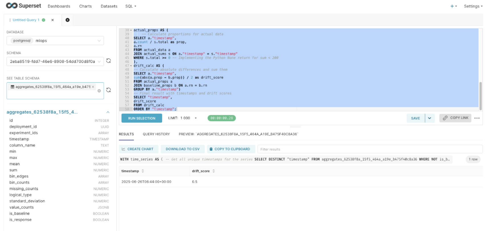

   

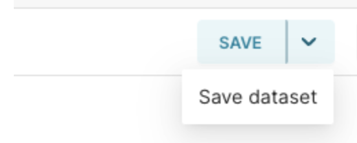
6. To save the result as a dataset, go to the Save drop-down and select Save dataset.
   

7. To convert it into a chart and add it to a dashboard:

   1. Go to Charts and customize the chart.
      
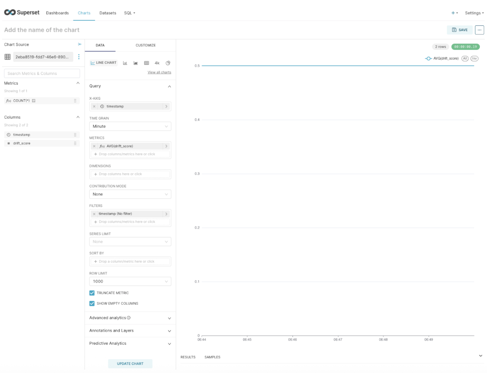
   2. Click Save, and add it to a dashboard.
      
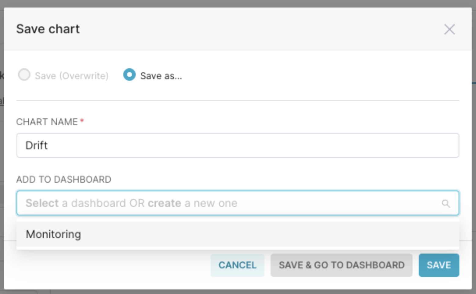
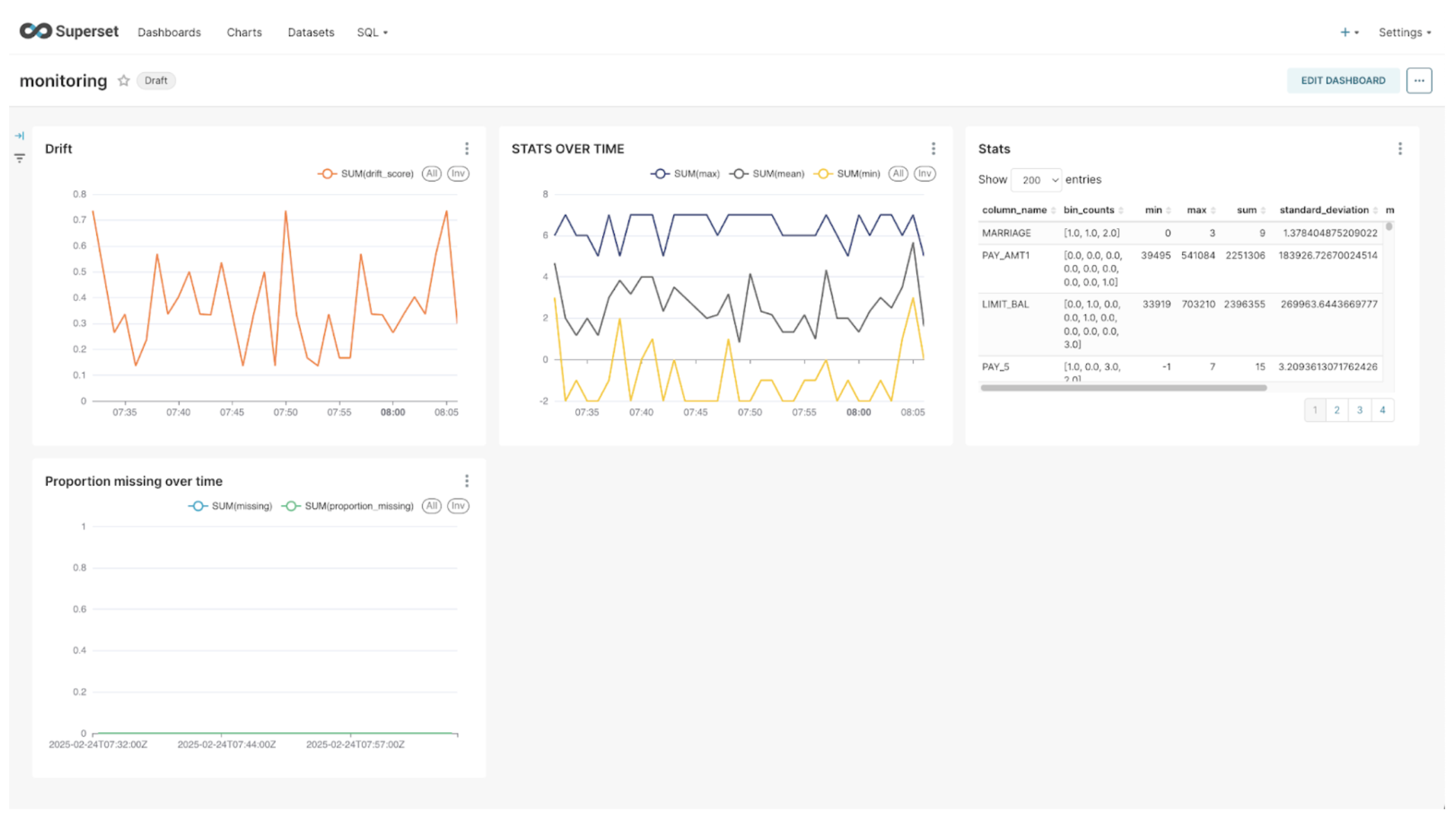
   3. Go to Dashboards and select the one you want to view.

You can explore more advanced dashboards for deeper insights.

Configure model monitoring with the Python client

To learn how to configure monitoring for your deployment using the H2O MLOps Python client, see Monitoring setup.

Raw data export to Kafka

Monitoring supports exporting raw scoring data to Kafka. This feature allows users to process scoring data in ways required by their internal regulations. Request and response data from scoring operations can be sent to a specified Kafka topic for downstream processing, auditing, or debugging. This feature is enabled by the MLOPs administrator.

During model deployment with monitoring enabled, scoring data and response data are sent to a default topic configured by the MLOPs administrator. Users can optionally specify a custom Kafka topic where the data are sent for this particular deployment. This allows separating data streams per deployment for improved observability. This configuration has no effect in case the Kafka intgration is disabled by the admonistrator.

note

The custom Kafka topic must exist before deploying the model. Monitoring will not attempt to create the topic automatically.

Once configured, the monitoring captures raw request and response data from scoring operations and forwards it to the configured Kafka topic (global or deployment-specific).

Common use cases for exporting raw data to Kafka include:

• Debugging and inspecting raw scoring payloads
• Auditing input/output for compliance
• Real-time analytics via stream processing systems

---

Feedback

• Submit and view feedback for this page
• Send feedback about H2O MLOps to cloud-feedback@h2o.ai